Learning Data Placement with RLDP in Modern Distributed Storage Systems

RLRP: High-Efficient Data Placement with Reinforcement Learning for Modern Distributed Storage Systems

Modern distributed storage systems with massive data and storage nodes pose higher requirements to data placement strategies. And with emerged new storage devices, heterogeneous storage architecture has become increasingly common and popular. However, traditional strategies expose great limitations in the face of these requirements, especially do not well consider distinct characteristics of heterogeneous storage nodes yet, which will lead to suboptimal performance. In this paper, we present and evaluate the RLRP, which is a data placement strategy based on deep reinforcement learning (RL). RLRP constructs placement and migration agents through the Deep-Q-Network (DQN) model to achieve fair distribution and adaptive data migration. Besides, RLRP provides optimal performance for heterogeneous environment by an attentional Long Short-term Memory (LSTM) model. Finally, RLRP adopts Stagewise Training and Model fine-tuning to accelerate the training of RL models with large-scale state and action space. RLRP is implemented on Park and the evaluation results indicate RLRP is a high-efficient data placement strategy for modern distributed storage systems and. RLRP can reduce read latency by 10%~50% in heterogeneous environment compared with existing strategies. In addition, RLRP is used in the real-world system Ceph, which improves the read performance of Ceph by 30%~40%.

做难事必有所得

Abstract

现代分布式存储系统具有海量的数据和存储节点，对数据放置策略提出了更高的要求。 而随着新型存储设备的出现，异构存储节点变得非常普遍和流行。 然而，传统的策略在面对这些需求时暴露出很大的局限性，特别是没有很好地考虑异构存储节点的鲜明特性，这将导致性能不佳。 本文提出并评价了基于深度强化学习(RL)的数据分布模型RLRP策略。 RLRP通过Deep-Q-Network (DQN)构建布局和迁移agent模型，实现公平分布和自适应数据迁移，克服了现有数据分布策略的局限性。 此外，RLRP通过注意机制为异构环境提供最佳性能。 最后，RLRP采用分段训练和模型微调的方法，加快了具有大规模状态和动作空间的RL模型的训练。 在Park上实现了RLRP，评价结果表明，RLRP是现代分布式存储系统中一种高效的数据放置策略，在异构环境下，与现有策略相比，RLRP可以降低30%~50%的读时延。 另外，在现实系统Ceph中使用了RLRP，使Ceph的读性能提高了30% ~ 40%。

Modern distributed storage systems with massive data and storage nodes pose higher requirements to data placement strategies. And with emerged new storage devices, heterogeneous storage nodes are very common and popular. However, traditional strategies expose great limitations in the face of these requirements, especially do not well consider distinct characteristics of heterogeneous storage nodes yet, which will lead to suboptimal performance. In this paper, we present and evaluate the RLRP, which is a data placement strategy based on deep reinforcement learning (RL). RLRP constructs placement and migration agents through the Deep-Q-Network (DQN) model to achieve fair distribution and adaptive data migration. Besides, RLRP provides optimal performance for heterogeneous environment by an attentional Long Short-term Memory (LSTM) model. Finally, RLRP adopts Stagewise Training and Model fine-tuning to accelerate the training of RL models with large-scale state and action space. RLRP is implemented on Park and the evaluation results indicate RLRP is a highly efficient data placement strategy for modern distributed storage systems. RLRP can reduce read latency by 10%~50% in heterogeneous environment compared with existing strategies. In addition, RLRP is used in the real-world system Ceph, which improves the read performance of Ceph by 30%∼40%.

降低最多50%的读延迟

addresses the challenges of training RL models.

Introduce

• （数据放置对分布式系统可靠性非常重要）

新兴的的大规模分布式存储系统面临着在数十甚至是数百数千的存储设备之间分发PB这个数量级别数据的艰巨任务

我们用数据对象指代存储系统中某一层次的数据单元，它可以理解为传统文件的分片，也可以理解为数据块组，也可以理解为面向对象存储系统中的对象。当存储系统的容量达到PB（10 5B）规模时，系统中维护的数据对象个数将达到10 9级别，包含数以万计的具有不同服务功能的存储节点，在这种规模下如何将数据对象按照存储节点的服务能力映射到各节点上成为一个很复杂的问题。

massive amounts of data

随着数据的爆炸式增长，新兴的的分布式存储系统数据量增大，集群规模大，这在性能、可扩展性和可靠性方面都有巨大的挑战。其首要任务是，在数万或数十万个存储设备中分配pb级的数据。这需要设计一种高效、公平、自适应的数据分布算法。不好的数据分布算法往往会导致数据的资源使用的不平衡，系统的一部分容易成为不必要的瓶颈，导致更长的延迟、更低的系统容量和更低的可用性。

With the explosive growth of data, emerging distributed storage systems with massive amounts of data and larger clusters are facing great challenges in performance, scalability and reliability. The primary task is to distribute petabytes of data among tens or hundreds of thousands of storage devices. It’s necessary to design an efficient, fair and adaptive data placement algorithm. Poor data placement algorithms often lead to imbalance in resource usage, which make part of the system becoming an unnecessary bottleneck, leading to longer delays, wasted storage space, and diminished reliability.

现代分布式存储系统给数据分布算法带了更高的要求和挑战，1）除了数据量和存储设备的增加，对存储资源的分布均匀，同时保证时间和空间高效，更加困难。2）随着时间的推移，分布式存储中会不断地加入新设备和删除旧设备。扩容和数据迁移是非常常见的，一个可扩展的数据管理方法是必须的，能够根据存储规模的变化调整数据的布局, 基于很少数量的数据迁移重新使得数据的均匀分布。3）设备发生失效的可能性更大。 在 PB 级的文件系统中, 设备失效几乎每天都会发生, 如此频繁的失效导致严重的数据丢失[ 2] 。所以数据算法必须提供一定的容灾机制，常见的包括副本复制和纠删码等等。4）另外设备异构性，随着存储设备的不断发展，更多高性能低延迟的存储设备在使用不同节点被使用。每个节点存储能力存在差异，这包括容量、网络、IO带宽等等。 算法应该综合考虑节点异构性，合理分布使系统达到最佳性能。这些需求给数据分布算法提出了很大的挑战。

实现可扩展和可靠的数据管 理之关键是设计一个能够自适应存储规模变化 公平 冗余 和高可用的数据布局算法, 能够在设备间公平地分布数据, 当存储设备集合改变时迁移最少的数据量, 同时提供冗余 机制提高数据的可靠性, 以及最大化系统的可用性等

Modern distributed storage systems have the following characteristics, which bring higher requirements and challenges to data placement algorithm. 1) Larger data volume and larger number of nodes. It is more difficult to distribute storage resources fairly, while ensuring time and space efficiency. 2) System scalability. Expansion and data migration are very common in modern distributed storage systems. A scalable algorithm is necessary, which can adjust the placement of data in response to changes in storage scale, and re-distribute data fairly with a small number of data migrations. 3) Higher reliability requirements. In the petabytes-level storage system, devices failures occur almost every day, and frequent failures cause serious data loss[??]. Therefore, the algorithm must provide disaster recovery capability, such as data replication and erasure codes, etc. 4) Heterogeneous storage nodes. With the development of storage devices, more high-performance and low-latency storage devices, such as non-volatile memory (NVM), NVMe and Optane SSD, are used in different nodes. The storage capacity of each node is different, which includes capacity, network, IO bandwidth, and so on. The algorithm should comprehensively consider the heterogeneity of nodes and reasonably distribute the nodes to achieve the best performance of the system. These requirements pose great challenges to the data placement algorithm.

传统算法在现代分布式存储系统表现出很大的局限性，往往顾此失彼，很难满足这些需求。最具代表性的数据分布包括：1）集中式的映射，它提供数据块和存储系统之间的映射（以表或者目录形式），用于定位数据项和复制。被许多文件系统例如GFS和HDFS等等采用。然而随着数据量增多，表或者目录会线性增长，导致存储空间开销和查找数据所需的开销会越来越大。2）以hash算法为代表的去中心化的映射方式，基于散列的数据放置方案通过提供数据和服务器之间的确定性映射，消除了维护全局映射的成本。常见的包括hash-based：线性hash【？】、可拓展hash[?]、rush、一致性hash[?]、crush[?]、random slicing等等，在分布式系统中得到广泛的应用。比如，Amazon的Dynamo系统通过虚拟节点优化一致性hash，保证系统高可扩展性和高性能。Ceph采用伪随机CRUSH算法，提供很高的灵活性和可靠性。但是它们在现代分布式系统中也有很大的缺陷，以CRUSH为例，因为副本的选择机制，数据平衡性较差且存在不可控的数据迁移。[?] 另外这些算法并没有考虑设备异构性，或者只考虑了部分差别，比如节点的容量等，这在现代存储系统中难以发挥异构节点最佳性能。

3）综合两则

Traditional algorithms make trade-offs on these requirements and show great limitations in modern distributed storage systems. The most representative data distribution mapping algorithms include: 1) Global mapping strategies provide a global mapping （a table or directory）between data blocks and storage systems for locating data items and replicas, which are adopted by many distributed file systems, such as GFS[?], HDFS[?] and so on. However, as the amount of data increases, tables or directories grow linearly in the number of data blocks, resulting in higher storage space and data search costs. 2) Decentralized mapping represented by the Hashing. Decentralized mapping schemes for data placement eliminate the cost of maintaining global mappings by providing a compact function (hashing, pseudo-hashing, etc.) between data and servers. Hash-based schemes including Linear hash[?] , Extensible hash[?] , rush, consistency hash[?] , crush[?] and random slicing, etc. are widely used in distributed systems. For example, Amazon’s Dynamo system optimizes the consistent by hash virtual nodes to achieve high scalability and Ceph uses the pseudo-random CRUSH algorithm to provide high flexibility and reliability. But they also have big flaws in the modern storage environment. Take CRUSH as an example, Its replica selection strategy often results in unbalanced data placement and uncontrolled data migration. In addition, these algorithms do not consider the heterogeneity of devices, or only consider some differences, such as the capacity of nodes, which makes it difficult to achieve the best performance of heterogeneous nodes in modern storage systems.

the storage space and the cost of finding the data will become more and more expensive it is difficult to meet these requirements because they tend to catch one and lose another. A scalable data placement method is necessary, which can adjust the layout of data according to the changes in storage scale, so that data can be stored in new devices. Re-distribute fairly on the set and control the smaller amount of migrationMany academic studies and industrial projects have tried to propose lots of excellent data placement algorithms.

1）被广泛使用的是（called Global mapping）2）以hash函数为代表的去中心化的映射方式，他们不维护3）是综合两种方式，但是这些研究在面对负载多变的现代分布式存储中存在各种问题，往往在 trade-off。另外由于要支持副本以及存储节点的异构性，很多算法处理不了，造成系统性能瓶颈。或者为了达到最高性能，资源往往集中于高性能的节点上，造成性能热点问题，导致。大规模的设备

the replica placement problem is a combinatorial optimization problem

很多研究表明，现代存储系统中带副本的数据分布问题，可以看成是组合优化问题。近年来，通过不断发展，RL在被用于解决各种系统问题，是被认为是解决组合优化问题的很好的方法。为此我们提出了RLDP，一个基于强化学习的数据分布算法，该策略试图通过结合基于表和伪随机哈希策略的经验教训，克服当前数据分布策略的局限性，解决RL模型的挑战，并且为复杂的异构系统提供优化性能。

公平的、冗余的、自适应的、高可用的、高效的数据分布算法，能够很好的满足现代分布式存储系统的各种需求。并且解决了

Many studies have shown that the data distribution problem with replicas in modern storage systems can be regarded as a combinatorial optimization problem. In recent years, Reinforcement Learning (RL) is widely used to solve various system problems and provide a good way to solve combinatorial optimization problems. Therefore, we propose RLRP (RL-based Replica Placement), a new data and replica placement scheme with RL models in modern distributed storage systems. This strategy overcomes the limitations of current data distribution strategies by incorporating lessons learned from table-based and pseudo-randomized hashing strategies. In addition, RLRP uses RL models to overcome the limitations of current data distribution strategies and addresses the challenges of training models, and provides optimal performance for heterogeneous systems. The main contributions of our paper are summarized as follows:

• 我们提出了基于强化学习的数据分布和数据迁移算法，提高了存储系统的
• 我们提出基于强化学习的
• 我们为异构环境设计了
• 我们在真实系统中使用我们的框架

The rest of this paper is organized as follows. Section 2 describes the background and motivation behind our work. We introduce the design and implementation details of RangeKV in Sections 3 and 4. Section 5 presents our comprehensive experiments and evaluation result analysis. Related work is discussed in Section 6. Finally, Section 7 concludes the paper.

Background and Motivation

• Data Placement Algorithm

分布式系统中，数据分布算法的任务是将数据分发到各个设备中，这可以看成是一个“balls into bins” model的典型案例。后面我们用数据对象指代存储系统中某一层次的数据单元，它就是“balls into bins” model中的ball。在存储系统中，它是数据分配和访问的单元，它可以代指传统文件的分片，可以指数据块组，也可以理解为面向对象存储系统中的对象。存储系统由大量后端存储节点(称为数据节点，DNs)组成，每个后端存储节点具有一个或多个cpu、本地内存和本地连接的存储数据的设备。 它们是“balls into bins” model中的“bins”。 因此，数据分布任务就是，接受可以创建对象的前端客户端的指令，将对象分配到数据节点中。根据现代分布式存储的特点，数据放置方案可以根据以下标准进行比较:

1）公平性:如果一个方案允许存储在数据节点上的对象的比例等于(或至少接近)它在系统总容量中所占的份额，则该方案称为公平的。公平性可以用数据节点的相对权重(对象数量除以权重)的标准差来衡量。

2）自适应性：如果一个方案在系统规模变化时，可以以最小迁移数据量达到系统重新均匀分配，则该方案可以称为自适应的。自适应性可以由系统规模变化时算法迁移的数据量与最优迁移的数据量之比值来衡量。

3) 冗余:一个方案在存储数据时采用了多个副本或擦除码，称为冗余。

4) 一个方案应该能够考虑数据节点的异构性，考虑节点负载性能等多种因素，以实现系统最佳性能。

5）时间和空间效率。 如果一种方案能以较低的时间和空间复杂度计算目标的位置，我们称其为时间和空间高效的方案。 ）

In distributed storage systems, the task of the data placement algorithm is to distribute data to various devices, which can be regarded as a typical case of the “balls into bins” model. In the following we use a data object (or just object) to refer to each logical data, which is the “ball” in the “balls into bins” model. the storage system, it is a unit of data allocation and access. It can refer to a traditional file fragment, a data block group, or an object in an object-based storage. The storage systems consisting of a large number of back-end storage nodes (called Data Nodes, DNs), each with one or more CPUs, local memory, and locally attached devices for storing data. And DN is the “bin’’ in the ``balls into bins” model. Therefore, the task of the data placement strategy is to take the instructions from front-end clients and distribute objects to Data Nodes. Clients of the system can read, create, and update objects. Based on the characteristics of modern distributed storage, the data placement scheme can be compared based on the following criteria:

1) Fairness: A scheme is called fair if it allows the fraction of objects stored at a data node is equal (or at least close) to its share of the total capacity of the system. Fairness can be measured by the standard deviation of the relative weight (the number of objects divided by weight) of the data nodes.

2） Adaptivity: A scheme is called adaptive if it can achieve fair redistribution with the near-minimum amount of migrated data in the case that there is any change in the number of objects, data nodes, or the capacities of the system. The adaptivity can be measured by the ratio of the amount of data migrated by the scheme to the amount of data optimally migrated In theory when the system scale changes.

3) Redundancy: A scheme can be called redundant if it adopts multiple replicas or erasure codes when storing data.

4) High Performance means that a scheme can consider data node heterogeneity including the node load, network bandwidth, etc. to achieve the best performance of systems.

5) Time and Space Efficiency. We call a scheme time and space efficient if it can compute the position of an object with a low time and space complexity.

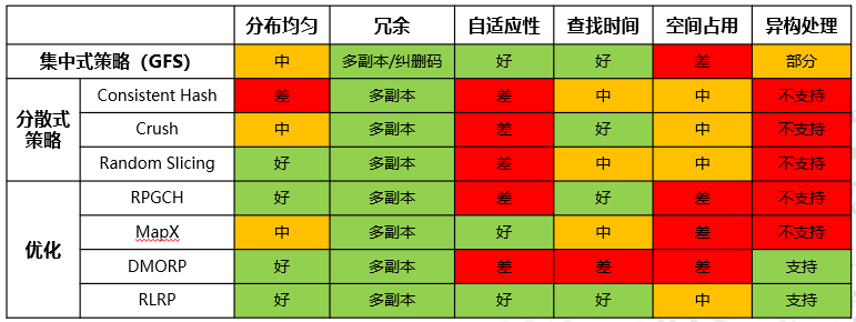
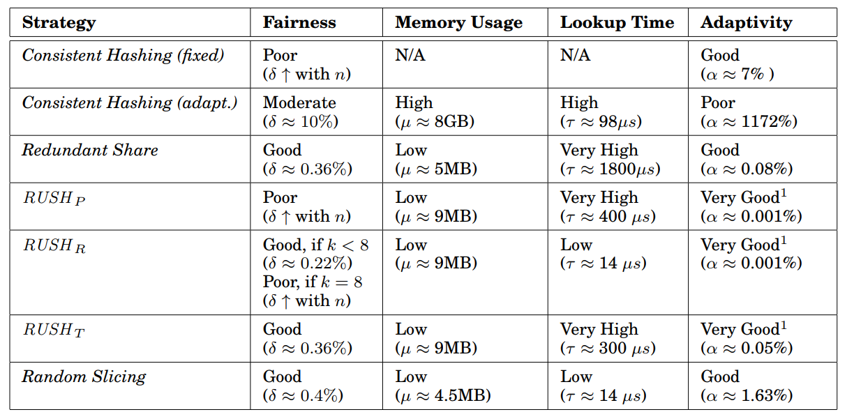
根据这些标准，传统算法有很大的局限性。table-based，consistent hash，crush，Random Slicing，ASURA 为对比对象，标准时good，Moderate，

It should be possible to schedule based on device availability adjust the location of data to maximize the performance of the system.The layout algorithm makes the percentage of data on each device equal to its relative weight, so the layout algorithm is fair

1）均匀性，2）传统算法的局限性。在我们的测试中，我们对传统算法的典型代表（。。。）进行了测试，如表？？。

强化学习是机器学习的一个领域，它关注的是人工代理应该如何在特定环境中采取行动，并以累积奖励概念最大化为目标。一个基本的RL模型由agent和环境构成，并且状态、动作、策略和汇报组成其基本要素。具体的，智能体在每一步的交互中, 都会获得对于所处环境状态的观察（有可能只是一部分）, 然后决定下一步要执行的动作。环境会因为智能体对它的动作而改变, 也可能自己改变。智能体也会从环境中感知到奖励信号, 一个表明当前状态好坏的数字。智能体的目标是最大化累计奖励, 也就是回报。强化学习就是智能体通过学习来完成目标的方法。

Reinforcement Learning[?] is an area of machine learning concerned with how artificial agents ought to take actions in a certain environment with with goal of maximizing some notion of cumulative reward. RL problems can be formulated as a Markov decision process (MDP), which is used to describe the process of interaction between agent and environment, and the State (S), Action (A), Reward (R) constitute its basic elements. Specifically, In RL, the environment is the world that the agent lives in and interacts with. At every step of interaction, the agent sees a (possibly partial) observation of the state of the world, and then decides on an action to take. The environment changes when the agent acts on it, but may also change on its own. The agent also perceives a reward signal from the environment, a number that tells it how good or bad the current world state is. The goal of the agent is to maximize its cumulative reward. The RL method are a way that the agent can learn behaviors to achieve its goal.

总的来说RL可以分为基于价值和基于策略的方法。基于价值的方法输出所有动作的收益，并选择最高收益的策略，显然它仅限于离散的动作空间。而基于策略方法是适用于连续的动作空间，他的输出是策略而不是具体的值，可以根据策略直接选择动作。在我们的问题中，动作空间是离散的，因此the value-based method被采用。

In general, RL can be divided into two categories: value-based and policy-based method. The value-based method outputs the value or benefit (generally referred to as Q-value) of all actions and chooses the action with the highest Q-value, obviously limited to discrete action spaces. The policy-based method is applicable to the continuous action space, and its output is a policy rather than a value, and the action can be immediately outputted according to the policy. The policy-based method is sufficient because of the discrete action space in RLDP.

Q- learning和Deep Q Network (DQN)是最经典的基于值的RL方法。Q-learning使用Q-table记录行为值 (Q value) , 每种在一定状态的行为都会有一个值 Q(s, a)，通常是状态和动作的二维表。策略就是每次根据状态选择Q表中最大Q-value的动作。

Q value的更新是根据贝尔曼方程：

其中r为从状态st移动到状态st+1时所获得的奖励，a为学习率0 < a≤1。 当g = 1时，Q函数等于奖励之和，当g = 0时，Q函数只考虑当前奖励。 当状态st+1为最终或终结状态时，算法的一集结束。 然而,q学习的

Q-Learning and Deep Q Network (DQN) are the most classic value-based RL methods. Each action in a certain state will have a value (Q-value), which are defined as Q(s, a). Q-learning records Q-value by a Q-table, which is usually a two-dimensional table of states and actions. The policy is to choose the action, which has the maximum Q-value in the Q-table, according to the state. Q-value will be updated at each step according to the Behrman equation:
\(Q(s_t, a_t) \gets Q(s_t, a_t) + \alpha[r + \gamma max_{a_{t+1}} Q(s_{t+1}, a_{t+1})-Q(s_t, a_t)]\) where $\alpha$ is the learning rate, 0 $\textless$ $\alpha \leq$ 1; r is the reward received when moving from the state $s_t$ to the state $s_{t+1}$; $\gamma$ is a discount factor, which favors short-term reward if close to zero and strives for a long-term high reward when approaching one.

In RLDP，采用DQN代替Q-learning，是因为Q-learning难以解决大规模分布式系统中数据放置问题中存在的状态空间大的问题。 DQN在q学习中使用神经网络而不是q表来评估q值，即：

其中w表示神经网络的参数。这是一种Function Approximation方法，然而，当使用神经网络等非线性函数逼近器来表示 Q 时，强化学习是不稳定或发散的。 这种不稳定来自观察序列中存在的相关性，事实上，对 Q 的小更新可能会显着改变代理的策略和数据分布，以及 Q 和目标值之间的相关性。经验回放被，它使用先前动作的随机样本而不是最近的动作来进行。[2]这消除了观察序列中的相关性并平滑了数据分布的变化。迭代更新将 Q 调整为仅定期更新的目标值，进一步减少与目标的相关性。

Deep Q Network (DQN) is adopted instead of Q-learning because Q-learning is hard to solve the problem of a large state space, which occurs in data placement problems in large-scale distributed systems. DQN uses neural networks rather than Q-tables in Q-Learning to evaluate Q-value,which can be described as follows:

[Q(s, a, w)\approx Q(s, a)]

where $w$ of $Q(s,a,w)$ represents the weights of neural network in DQN. This is a Function Approximation technology\cite{dqn}. However, when a nonlinear function approximator such as a neural network is used to represent Q-value, reinforcement learning is unstable or divergent, which comes from the correlations present in the sequence of observations, the fact that small updates to Q-value may significantly change the policy of the agent and the data distribution, and the correlations between Q-value and the target values. Experience replay uses a random sample of prior actions instead of the most recent action to proceed and is a common optimization technique for DQN. Experience replay removes correlations in the observation sequence and smooths changes in the data distribution. Iterative updates adjust Q towards target values that are only periodically updated, further reducing correlations with the target.

The technique used experience replay, a biologically inspired mechanism that uses a random sample of prior actions instead of the most recent action to proceed.[2] This removes correlations in the observation sequence and smooths changes in the data distribution. Iterative updates adjust Q towards target values that are only periodically updated, further reducing correlations with the target.

• Challenges

据我们所知，我们是第一个使用强化学习来优化存储系统数据分布的算法，这将面临非常大的挑战：1）如何对问题进行建模，如何定义强化学习各要素？2）如何处理迁移问题？3）当节点数和数据量比较大的情况下，如何加速训练？4）异构环境，如何兼顾性能和均衡性？RLDP很好的解决了这些问题，为强化学习解决系统问题提供了很好的案例。

this is the first work using reinforcement learning to optimize the data distribution of storage systems, which will face daunting challenges : 1) How to model the problem and how to define the elements of reinforcement learning? 2) How to deal with migration issues? 3) How to speed up training when the number of nodes and the amount of data are relatively large? 4) How to balance performance and fairness in a heterogeneous environment? etc. RLDP solves these problems well and provides a good case for reinforcement learning to solve system problems.

The problem, due to its generality, is studied in many other disciplines(e.g. game theory, control theory, etc). In the case of machine learning, the environment is typically formulated as a Markov Decision Process (MDP), as many reinforcement learning algorithms for this context utilize dynamic programming techniques. The main difference between reinforcement learning and the classical dynamic programming methods is that in RL do not assume knowledge of an exact mathematical model of the MDP. An advantage of RL algorithms is that they can target large MDPs where exact methods become impracticable.

Design

在本节中，我们将描述一种新的基于RL的数据分布方案，for现在分布式存储系统。我们首先对整个RLRP框架和RL模型进行介绍，其次我们对模型训练、异构环境处理以及实现进行详细的介绍。

In this section, a new RL-based data placement scheme for distributed storage systems will be described. The whole RLRP framework and RL models is introduced first. Then, the model training, heterogeneous environment processing and implementation are introduced in detail.

• RLRP System

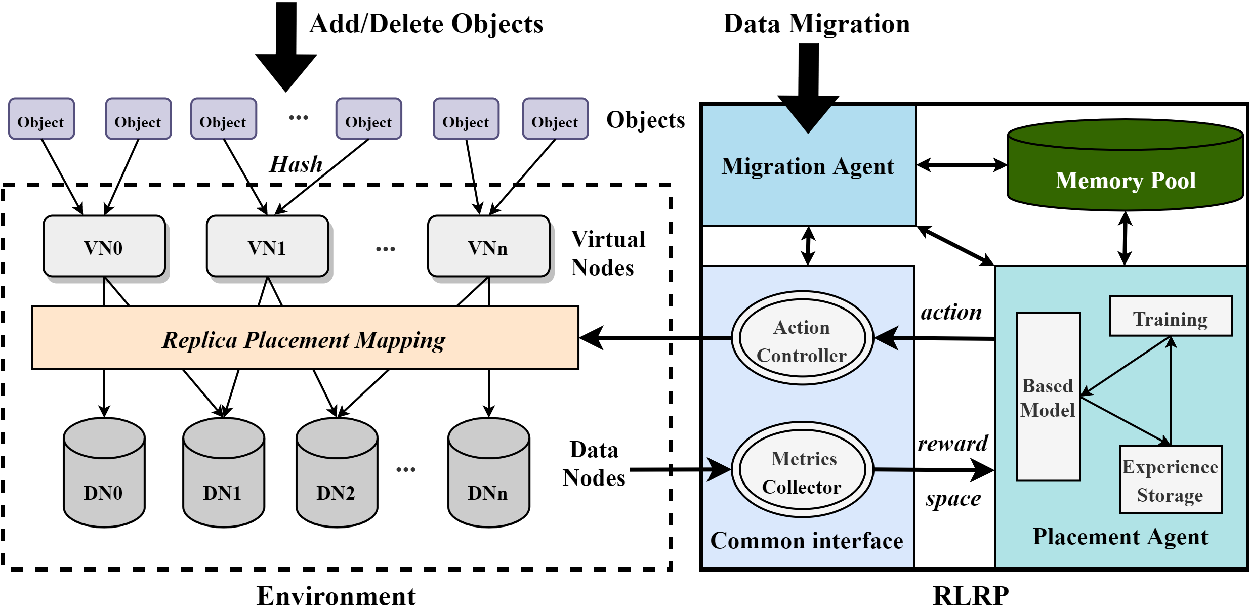
如图？？所示，整个RLRP框架定义了对象到数据的映射，提供接口完成上层对对象的各种操作，包括对象创建、删除和迁移等等。我们基于RL模型，定义了Environment和Agent基本元素。

The overall RLRP architecture is shown in Fig. \ref{RLRP}. The RLRP framework defines the mapping of objects to DNs (see Section ?) and provides interfaces for upper-layer operations on objects, including object creation, deletion, and migration. Based on the RL models, the basic elements of Environment and Agent are defined as follows.

Environment：如图？？，我们不直接分布objects到DNs，而是先映射对象到Virtual Nodes，这与Dynamo中的虚拟节点，Ceph中的归置组以及OpenStack-Swift中的分区具有相同的概念。系统上的每个数据对象通过一致性哈希函数映射映射到一个虚拟节点。散列函数应用数据对象的标识来计算使用虚拟节点总数的模运算，然后定义对象属于哪个虚拟节点。由于散列映射层的散列函数输出均匀分布的散列值，因此每个虚拟节点中的对象数量是平衡的。虚拟节点是管理对象、数据迁移和故障管理的基本单位，它设定可以很好解决对象数量大导致难以管理的问题，从而降低数据分布的难度。虚拟节点的个数通常在系统启动前设定，且不会轻易变化，否则会产生大量数据移动的副作用。默认情况下，假设数据节点数为N_DN，副本数是r，则初始化虚拟节点数计算如下：在计算出V后，虚拟节点数量等于V舍入到最接近2的N次幂的值。比如，副本数是3，当数据节点数分别为100，200，300时，V等于，3333.333333，6666.666667，10000，则虚拟节点数等于4096，8192，8192。

Instead of directly distributing objects to DNs, we first map objects to Virtual Nodes, which has the same concept of virtual nodes in Dynamo, placement group (PG) in Ceph, and partitions in OpenStack-Swift. Each data object is mapped to a virtual node through a hash function, which applies the identification (e.g. object ID or name) of a data object to calculate the modulo operation using the total number of virtual nodes, defining then which virtual node the object belongs to. The number of objects in every virtual node is balanced due to the hash function of the hash mapping layer that outputs hashed values uniformly distributed. The virtual node is the basic unit of object management, data migration, and fault recovery. It can ease the difficulty of managing the large number of objects, so as to reduce the burden of data distribution. The number of virtual nodes is set before the system starts and does not change frequently, otherwise it would create side-effect of huge data movements. By default, assuming that the number of data nodes is N_DN and the number of replicas is R, the recommended number of virtual nodes is calculated as follows: $V = 100 * N_d / R$, and $N_v$ is equal to $V$ rounded to the nearest power of 2. For example, if the number of replicas is 3, when the number of data nodes is 100,200,300, the V equals 3333.333333, 6666.666667, 10000, and the number of virtual nodes equals 4096,8192,8192.

VNs映射到DNs通过RLRP来决策，一个虚拟节点会在不同数据节点上复制多份，副本数由上层应用决定。并且由标志来分辨主副本所在，主副本是首先写入的节点，在复制到别的副本，也是读操作访问的节点。如图中例子，副本数是2，VN1选择副本存放的数据节点是DN1和DN2。当每个virtual node被创建后，RLRP算法会考虑DNs节点的状态，通过Agent算法选出副本，并将映射关系加到RPM中。每个对象的读操作首先是通过hash函数找到虚拟节点，在通过查找RPM查找VN所在的数据节点。由于经过hash分组，映射表不会像集中式那样随着objects增长而线性增长。由一个映射表存储。每次读将通过查表找VN所在位置。由于经过hash分组，映射表不会像集中式那样随着objects增长而线性增长。

A Replica Placement Mapping Table (RPMT) generated by RLRP is responsible for defining the mapping of virtual node replicas to data nodes. A virtual node is replicated multiple times on different data nodes and the number of replicas (the replication factor) is determined by the upper-layer application. In the example shown in Fig. \ref{RLRP}, the replication factor is 2, and VN1 selects DN1 and DN2 as the data nodes where the replicas are stored. RPMT can determine the location of the master replica, which is the node that is accessed by read operations and is first written and then copied to other replicas during the write process. When each virtual node is created, the RLRP will consider the states of the data nodes, select the data nodes by RL Agent, and add the mapping to the RPMT. The read operation for each object first finds the virtual node through the hash function, and then finds the data node by looking up the RPMT. Due to the grouping by virtual nodes, the table (RPMT) will not grow linearly in the number of objects like global mapping strategies.

Agent is the main body of RL model, divided into Placement Agent and Migration Agent, which make decisions for distribution and Migration respectively. The basic framework of RL Agent is shown in the figure?? For distribution and migration, we use two kinds of agents to deal with the problem of distribution and migration. The two agents use the same model framework, but the defined elements are different. The framework of each Agent is a standard DQN model, which uses MLP as its neural network model by default and RNN+Attention model in heterogeneous environment. Let’s first introduce the basic Placement Agent, which only considers DN capacity differences. Next, the basic migration Agent is introduced. Then it introduces how to accelerate the training and optimize the model. Finally, the construction of Placement model and migration model under Heterogeneous environment is introduced, which will consider various factors that affect performance. It should be noted that the framework of Agent in heterogeneous environment is the same, but the neural network model is different.

Common interface主要是RLRP和Environment交互的接口，包括Metrics Collector和Action Controller两部分。Metrics Collector负责从环境中获取系统性能和延迟，以及DNs节点的相关属性。DNs的相关属性将作为强化学习的样本特征，在不同环境可以有不同的选择，尤其是异构条件下，关键属性的选择是非常重要的。它们将作为RL Agent的状态和奖励信息送给Agent。

Action Controller负责实施Agent决定的action，它会通过更新映射表来决定选择的副本的数据节点或者迁移后的数据节点。

Common Interface is the interface between RLRP and Environment, including Metrics Collector and Action Controller. Metrics Collector is responsible for obtaining states and attributes of DNs, and system performance or latency from the Environment. The attributes of DNs will be used as the features of the training sample in RL, which can be selected differently in different environments. Especially under heterogeneous conditions, the key feature selection is very important. These metrics are sent to the RL Agent as the state information (st) and reward information (rt) respectively. Action Controller applies the actions of replica placement or data migration suggested by the RL Agent through updating the Replica Placement Mapping Table.

重新写!

Memory Pool 存储训练相关权重参数，包括DQN的经验回放，模型参数等等

Memory Pool stores training-related weight parameters, including DQN experience playback, model parameters, etc.

RL Agent是RLRP系统的核心，可以看作是RLRP系统的大脑，它从环境中接收奖励和状态，并更新策略来指导如何分配副本以获得更高的奖励。RL Agent基本框架如图？？,Agent分为Placement Agent和Migration Agent，分别为分布和迁移做出决策。数据迁移是指当存储规模发生变化时（数据节点增加或者减少），数据或副本调整以达到数据重新平衡。两者Agent使用一样的模型框架，一个标准的DQN模型，只是定义的元素不同。另外，Agents在异构和非异构的环境下DQN中神经网络模型有所区别。它默认使用的MLP作为其神经网络模型，在异构环境中使用RNN+Attention模型。在非异构环境中，基本的Placement Agent和迁移Agent只考虑DN的容量区别，而Heterogeneous环境下它会考虑各种影响性能的因素。为了加快RL训练，Agent可以并行生成经验(在内存池中存储经验)，并在经验缓冲区达到批大小后进行经验重放，以进行训练和参数更新。

RL Agent can be regarded as the brain or core of the RLRP system, which receives reward and state from Environment and updates the policy to guide how to distribute replicas for getting higher reward. AL shown in the figure?? , agents consist of Placement Agent and Migration Agent, which make decisions for distribution and migration respectively. Data migration refers that when the storage scale changes (data nodes increase or decrease), data or replicas are adjusted to achieve fair redistribution. The two agents use the same model framework, which is a a standard DQN model, but the elements defined are different. To to speed up RL training, Agent can generate the experience in parallel (experience storage in Memory Pool) and perform experience replay when the experience buffer reaches the batch size for training and parameter updating. In addition, the neural network models of DQN are different in heterogeneous and non-heterogeneous environments. MLP is used as the neural network model by default, while LSTM (an RNN model) with Attention mechanism is used in heterogeneous environment in the DQN model of agents. In the non-heterogeneous environment, the basic Placement Agent and Migration Agent only consider the capacity difference of DNs, while various factors that affect performance will be considered in the Heterogeneous environment.

接下来，我们先介绍非异构环境下1）basic Placement Agent and 2）Migration Agen，然后介绍3）模型的训练加速，以及4）异构条件下的模型构建，最后介绍5）实现.

Next, we first introduce basic Placement Agent, Migration Agent and training optimization of the model in non-heterogeneous environments. The model in heterogeneous environment and the implementation will follow.

In this simulated environment, an RL agent balances jobs over multiple heterogeneous servers to minimize the average job completion time. Jobs have a varying size that we pick from a Pareto distribution (Grandl et al., 2016) with shape 1.5 and scale 100. The job arrival process is Poisson with an inter-arrival rate of 55. The number of servers and their service rates are configurable, resulting in different amounts of system load. For example, the default setting has 10 servers with processing rates ranging linearly from 0.15 to 1.05. In this setting, the load is 90%. The problem of minimizing average job completion time on servers with heterogeneous processing rates does not have a closed-form solution (Harchol-Balter & Vesilo, 2010); a widely-used heuristic is to join the shortest queue (Daley, 1987). However, understanding the workload pattern can give a better policy; for example, one strategy is to dedicate some servers for small jobs to allow them finish quickly even if many large jobs arrive (Feng et al., 2005). In this environment, upon each job arrival, the observed state is a vector (j;s1;s2;:::;sk), where j is the incoming job size and sk is the size of queue k. The action a 2 f1;2;:::;kg schedules the incoming job to a specific queue. The reward ri = Pn [min(ti;cn)-ti-1], where ti is the time at step i and cn is the completion time of active job n.

• Placement Agent

在与环境交互的每一步，Placement Agent根据当前DNs的状态，决定VN副本放置的动作，之后计算reward反馈回agent。每一步交互就是确定每一个VN的存储副本的DN。假设存储系统的数据节点数量是n，在计算第i个VN（VNi, 也可以说是step i）的副本位置时，我们的问题的State-action-reward结构可以描述如下。

At each step of interacting with the environment, according to the current state of DNs, Placement Agent determines the action of placing replicas for each VN, and then the reward is calculated and fed back to the agent. Let n be the number of data nodes in the system. When calculating the replicas location of the ith VN (VNi, ), the State-action-reward configurations of our problem can be described as follows.

状态空间表示在考虑VNi时刻（称为i时刻）的数据节点负载状况，即所有数据节点的相对权重的列表{w0, w1,…,wn}，其中wk等于i时刻DNk中VN总数除以DNk的容量，表示相对的负载状况。

We describe state at time step t as st, which means the load state of data nodes when considering VNt. St can be defined by the

the list of relative weights of all data nodes:

St = {w0, w1… Wn}

where wk is equal to the total number of VNs in DNk time step t divided by the capacity of DNk, indicating the relative load state.

action：动作空间是{DN0，DN1，DN2，，，DNn}，表示副本可选择的数据节点编号。At for VNt 等于k元组（DN，DN，，，DN），表示VNt的k个副本所在节点。其中第一个为主副本，具体副本选择算法后面会介绍。默认情况下，选出来的数据节点互不相等以提高可靠性，但是如果n小于K，则会有重复副本在同一节点的情况。

The set of actions is represented by A = {DN0，DN1，DN2，，，DNn}，indicating the numbers of all data nodes. We define action at time step t by the following k tuple At = (DN,DN,..,DN ), which represents the data nodes where k replicas of VNt are stored. The first one is the master replica, and the specific replica selection algorithm will be described later. By default, the selected data nodes are not equal to each other to improve reliability, but if n is less than K, there will be duplicate replicas on the same node.

reward：我们用STD表示St的标准差，直接反映了此刻节点的均衡性。Rt等于St的标准差的负数，即Rt = - STD。St的标准差越大，表示节点越不均衡，Rt就越小，反之Rt越大，越能激励agent往标准差小的方向分布虚拟节点。

We use STD to represent the standard deviation of St, which directly reflects the balance of nodes at the moment. Rt is equal to the negative of the standard deviation of St, which is Rt = -std. The larger the standard deviation of St is, the more imbalanced the nodes are, and the smaller Rt is. Conversely, the larger Rt is, the more agent can be motivated to distribute virtual nodes in the direction of small standard deviation.

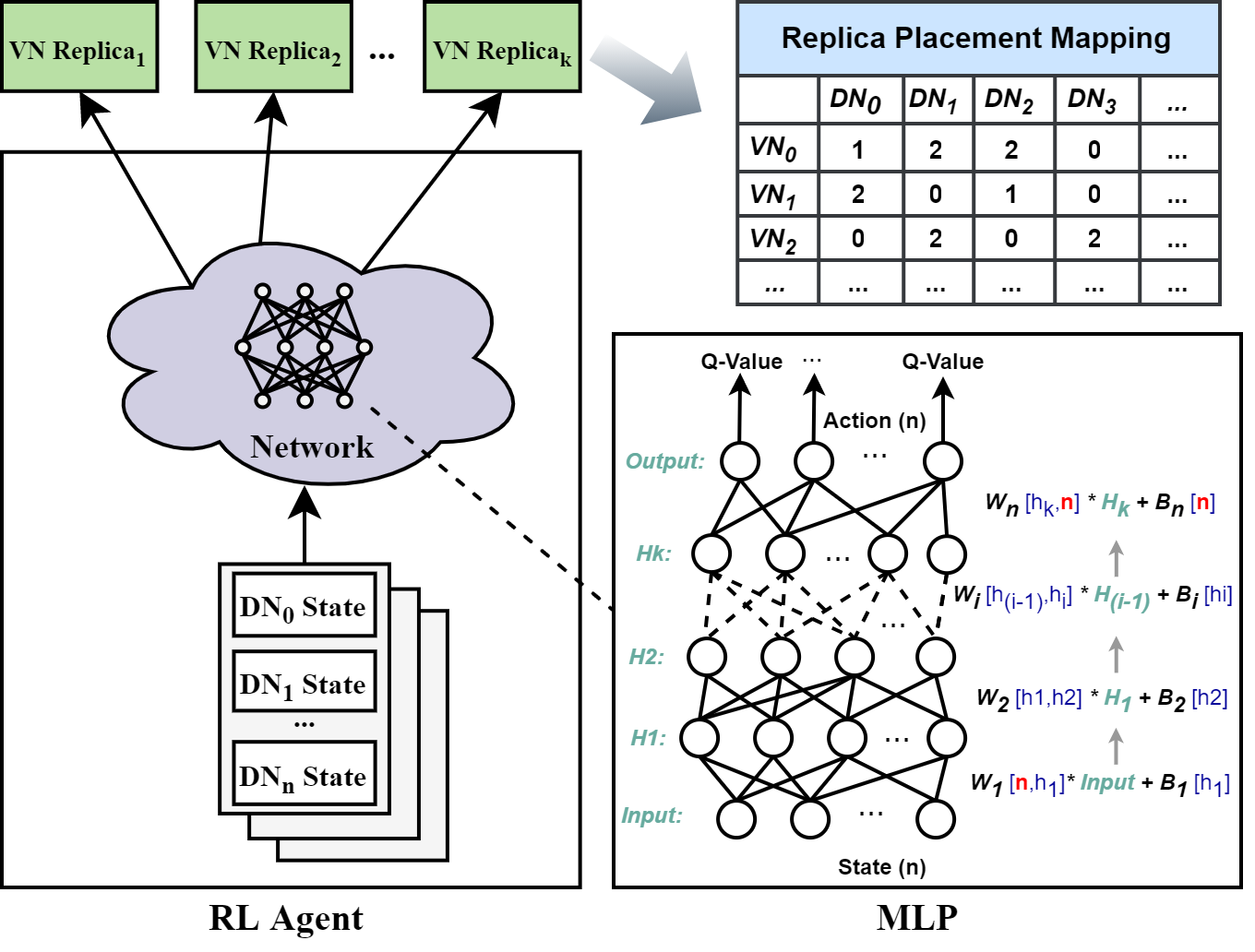
如图2，Placement Agent的输入是每个数据节点的负载状况 ，而输出是k个副本，它们会被加入到映射表中。Replica Placement Mapping是一个二维的映射表，{0，1，2}，其中1表示该虚拟节点的主副本所在，2表示其他副本。默认情况下Placement使用2x128个节点的MLP，即两个隐藏层，每个128个节点。具体模型节点配置可以根据实际环境被设置。

副本放置算法具体描述了Placement Agent流程。列表a_list被使用来存储所有副本action，当a_list的长度达到副本数时，算法停止。在默认的，数据节点数大于副本数情况下，a_list中不能存在相同元素。所以算法会优先选择Q值最大的作为action，选其他副本的action和以前某次一样，则选Q值次大的作为替补，以此类推。具体的，在xx行，动作选择是通过调用E函数实现，使用的时e-greedy策略，即以e概率随机选择action，否则从Q_value中由大到小以此选择action。

若数据节点小于副本数，则每次副本选择不会考虑是否有重叠，这种情况一般不会出现在现实中，未在算法中显示。每次选出action之后，调用u函数来实施放置动作，并且更新数据节点状态和映射表，并根据新状态计算标准差作为奖励，和新状态一起返回。元组《》会被存储到the replay memory D中, 可以在训练流程中用于agent的训练和神经网络参数更新。

Replica Placement Algorithm specifically describes the Placement Agent process. A list a_list is used to store all actions (numbers of data nodes for replica placement), and the algorithm stops when the length of a_list reaches the replication factor. By default, the number of data nodes is greater than the number of replicas, so the same elements cannot exist in a_list. Therefore, the algorithm will preferentially select the action with the largest value in Q_value. If the action is the same as that of the previous one, the action with the second largest value in Q_value will be selected as a substitute, and so on. Specifically, in line xx, action selection is achieved by calling the E function , which applies e-greedy method, that is, the action is randomly selected with probability e, otherwise the action is selected with the value from the largest to the smallest in Q_value. If the number of data nodes is smaller than the number of replicas, each action selection will not consider whether there is overlap, which generally does not appear in reality and is not shown in the algorithm. After each action is selected, the u function is called to perform the replica placement with a_list. The state of data nodes is update and returned as a new state, and mapping table is updated. The standard deviation calculated based on the new state is returned as a reward. A tuple “” will be stored in the Replay Memory D, which can be used for training agent and updating neural network parameters in the training process.

节点变化可以分为增加和移除节点两种情况。减少节点还是使用Placement Agent。具体的，假设移除了节点DNm，将DNm中的VN副本通过Placement Agent带有两个限制重新映射到其他节点。限制1：不能选择action DNm；限制2：当n>k时，不允许副本冲突，即不能选择的节点拥有该VN的副本。减少节点之后需要重新训练Placement Agent用于后续节点的分布。

Node changes can be divided into two situations: adding and removing nodes. Removing nodes still uses Placement Agent model. Specifically, assume that the node DNm is removed and the VN replicas in the DNm is remapped to other nodes via Placement Agent with two limitations. Limitation 1: DNm cannot be selected as action; Limitation 2: When n>k, replica conflict is not allowed. That is, the data node that has a replica of the VN cannot be selected. The reduction of nodes requires retraining of Placement Agent for subsequent node distribution.

• Migration Agent

用于增加节点，或者手动触发数据迁移，以优化系统的可适应性。当增加一个数据节点时，要对每一个虚拟节点考虑是否迁移副本到新节点上。当考虑第t个VN时， Migration Agent的State-action-reward配置和Placement Agent都是一样的，除了action，被如下描述：

Migration Agent is used for scenarios of adding nodes or manually triggering data migration, to optimize the adaptive of data placement. When adding a data node, it is need to consider migrating replicas to the new node for each virtual node. The State-action-reward configurations of Migration Agent is the same as that of Placement Agent, except for the Action, which is described as follows:

action: 动作集是0~k的常数集{0, 1, …, k}，action a的不同取值表示对每个VN的不同副本的迁移命令。如果a等于0，则VN不会迁移任何副本到新节点上。如果a等于1到k任意一个值i，则表示迁移VN的第i个副本到新节点中，需要从RPM找到。以三副本系统为例，动作空间A={0，1，2，3}.VNi的副本在(DNk, DNj, DNl)中，当action等于0时，VNi不进行任何副本迁移。副本DNk会被迁移当action取值1时，另外action为2，3时，副本 DNj, DNl将会被迁移到新节点中。

The action set is a constant set from 0 to k (). Different values of action a indicate migration commands for different replicas of each VN. If a is equal to 0, VN will not migrate any replicas to the new node. If a is equal to any value i from 1 to k, it means that the i-th replica of the VN is migrated to the new node, which can be found from the RPM. Take the system of three replicas as an example, the action space A={0,1,2,3}. The replicas of VNi is in (DNk, DNj, DNl). When action is equal to 0, VNi does not perform any replica migration. The replica DNk will be migrated when the action value is 1. And the action is 2 or 3, the replica DNj or DNl will be migrated to the new node.

通过上述action定义，可以保证新节点加入后一些虚拟节点的副本迁移到新节点中，并且还是以标准差作为奖励可以保证迁移结束后数据节点数据的均衡，符合适应性的要求。Migration Agent算法步骤和Placement Agent类似，另外再增加节点后，Placement Agent也需要重新训练。

Through the above action definition, it can be ensured that some replicas of virtual nodes are migrated to the new node after the new node joins in the system, and the standard deviation is still used as a reward to ensure the balance of data node data after the migration, which meets the requirements of adaptability. Migration Agent training is similar to Placement Agent. In addition, after adding nodes, Placement Agent also needs to be retrained.

• 训练加速

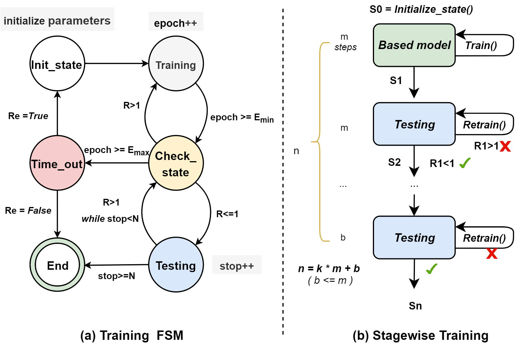
训练过程分成模型训练和模型测试两个阶段，我们构造一个有限状态机来控制训练，如图1所示。这训练有限状态机可以分成六个状态。初始化状态，用于初始化所有训练参数和agent模型的参数。初始化结束进入训练阶段，和传统的固定量训练迭代次数不同，训练有限状态机设定迭代次数的下限Emin和上限Emax。当训练迭代次数epoch达到Emin，进入Check状态，它用于检测训练效果。图中R表示训练后的数据节点状态标准差，用于反映训练效果，我们设定R小于等于1属于合格的结果。在Check状态计算R，如果训练不佳，重新回到训练状态在训练一周期再进入Check状态。如果R小于等于1，会进入测试阶段。测试中使用stop作为停止计数器，在每个测试周期后如果测试结果是合格的，stop会加1，否则返回Check_state。N是一个常数，只有在测试环节连续N次或以上达到要求才可结束。为了防止训练收敛不了，训练周期超过Emax，则会进到Time_out，此时训练会报错。参数Re表示是否重新开启训练（回到初始化阶段重新初始化新的参数），或者直接结束，这参数由用户自行设定。

As shown in Fig. 1 (a), a finite state machine (FSM) is constructed to control the training process, which is consists of model training and model testing. The training FSM can be divided into six states. Initialization state is used to initialize all training parameters and the parameters of the agent model. The training state is after initialization. Unlike the traditional fixed number of training epochs, the training FSM sets the lower limit Emin and the upper limit Emax of the number of epochs. When the number of training epochs epoch reaches Emin, it enters the Check state, which is used to check the quality of training. The standard deviation R of the data node status after training is calculated in Check state. A result can be called qualified only if R is less than or equal to 1. If the training is good, it’s turn to the testing state (), otherwise it’s back to training state. The testing state uses stop as a stop counter, and N is a constant. After each test epoch, stop is incremented if the test result is good, otherwise Check_state is returned. The training process can be completed only when the results is good for N consecutive times or more in testing state. In order to prevent the training from failing to converge, if the training epochs exceed Emax, it will enter Time_out state, at which time an error will be reported during training. The parameter Re specified by users indicates whether to restart the training (return to the initialization state to initialize the new parameters), or end directly. The following describes the training process of each epoch in detail.

这是经典的DQN训练算法。这与传统的DQN的目标值不同，它少了terminal state下的情况，因为在我们的环境中，并没有目标状态。Next, parameters () of Q network are upaded with the mini-batch stochastic gradient descent (SGD) method and minimize the training objective:

Algorithm \ref{alg:Training} lists the pseudo code of the training algorithm, which is the classic DQN training algorithm \cite{dqn}. Firstly the tuples in the relay memory $D$ are replayed periodically to generate mini-batches B. For each mini-batch transition $(s, a, r, s’)$ ($s’$ is the next state of $s$), the target value is calculated as follows: [y = r + \gamma max_{a’} Q(s’, a’; \theta)] where $\gamma$ a discount factor and $\theta$ is the weight vectors of $Q$ network. Different from the target value of the traditional DQN, it lacks the situation in the terminal state, because in our environment, there is no target state. Next, parameters ($\theta$) of $Q$ network are upaded with the mini-batch stochastic gradient descent (SGD) method \cite{playing} and minimize the training objective:

[ min L(\theta) = \mathbb{E}[y - Q(s,a; \theta))^2]] which is to minimize the expectation of the difference between the target value and the output of $Q$ network.

但是实际训练过程中，随着对象数增加，虚拟节点增加以及数据节点增加，为了达到前面提到的高要求，训练时间也增加很多。为了加速训练，两项优化被采用。分段训练用于优化虚拟节点增加的情况，而模型迁移用于数据节点增加的情况。另外在训练过程中，我们发现状态空间非常庞大，在我们的环境中，我们是以标准差来衡量状态的好坏，很多状态其实从这个角度看是一样的。比如考虑以下两种状态：（100，200，300），和（0，100，200）,他们标准差都是81.6496580928。这两者状态可以被认为是一致的，即在这两者状态下选择的action应该是一样的。于是在训练过程中，相对状态集被使用，原状态集中所有元素都减去最小元素。这样可以减少很多冗余的状态，但是在系统中还是要维护一个真实的负载状态。

However, in the actual training process, as the number of objects, virtual nodes and data nodes increases. In order to meet the high requirements mentioned above (R<=1), the training time also increases a lot. In order to speed up training, two optimizations are adopted. Stagewise Training is used to optimize training when virtual nodes increase, while Transfer Learning is used when data nodes increase. In addition, the state space will be very large during the training process. In our environment, standard deviation is used to measure the quality of the state and many states are actually the same from this perspective. For example, consider the following two states: (100, 200, 300) and (0, 100, 200), their standard deviations are both 81.6. The two states can be considered to be consistent, which means that the action selected in the two states should be the same. So the relative state set, which is obtained by subtracting the smallest element from all the elements in the original state set, is used in in the training process and can reduce a lot of redundant states. Of course, a real load state must be maintained in the system.

分段训练。由于一次epoch训练的步骤数等于VN的的数量。但是在现代存储系统中，对象数量是非常庞大的，尽管通过hash分组成虚拟节点，但这数量也是不小的。在实际训练中，如果选择较小样本则效果不佳，如果选择较大的样本则训练时间非常长。我们采用一种分段训练的方式。首先我们使用一个较大的样本数（图中的n）作为训练数据集，每次随机抽取一部分作为小样本（图中m），假设n=k*m+b，则总共可以分成k+1份样本，每个样本维护一个训练状态机。默认的，k设定为10，根据大样本的数量n可以算出m和b。如图所示，其中一份小样本从FSM的初始化阶段开始进行训练，训练完成的模型成为基模型。状态由S0变成S1，接着基于状态S1，训练将直接进入第二个小样本的训练状态机的测试状态。原状态是S0，训练完成以状态S1直接进入第二个样本的训练状态机的测试状态。如果测试结果合格，则进入下个样本阶段，否则在FSM中会回到训练阶段重新训练。以此类推，直到完成最后的样本测试。

Stagewise Training. In modern storage systems, the number of objects is very large, and the number of the virtual nodes is also large although grouped by hash. And the number of steps in an epoch training is equal to the number of virtual nodes. In practical training, if a small sample is selected, the training result is not ideal; if a large sample is selected, the training time is very long. To this end, as shown in Fig. 1, a segmented training method is adopted. Firstly, we use a larger number of samples (n in the figure) as the training data sets, and randomly divide into many small samples (m). Assuming n=k*m+b, the large samples can be divided into k+1 small samples in total. By default, k is set to 10, m and b can be calculated by the number of large samples n. Each sample maintains a TFSM. As shown in Fig. 3, a small sample with m size is trained from the initialization state of TFSM, and the trained model became the base model. The state changes from S0 to S1, and then based on state S1, base model will directly be test in the test state of TFSM in the second small sample. If the test result is qualified, it’s turn to the next sample stage, otherwise base model will be retrained in the training state of TFSM with the the second small sample. And so on, until the final sample test is completed.

模型微调。数据节点的增加从两个方面增大了训练难度：1）数据节点多导致训练时间长；2）数据节点增加，状态，动作空间和神经网络的维度变化，原模型不可用。如前面提到，每次节点数量变化都会导致Placement Agent的重训练，影响系统的恢复和性能。一种模型调整的方法被采用，当节点数量增加时，它可以基于旧模型更新神经网络结构来减少训练时间。具体的，当神经网络维度增加时，模型微调会使用旧模型的参数，作为新模型低维度的初始参数，新增维度置零或者随机初始化。

具体操作如下例子所示，假设我们有输入变量x ，其维度为dx，经过一个激活函数后得到向量 y = W1 x+B1，其维度为dy，然后再经过一层全连接层得到向量 z=W2 y + B2，其维度为 dz。如果需要增加向量y的参数量，增加其维度从dx到dy，那会导致W1, B1, W2的维度都发生改变： W1=[ W1 R()], B1= [B1 R()] W2= [W2, 0 ]这里R()指的是随机初始化，经过这个操作后，可以发现 W1’ B1’的前dy个权重和W1, W2是完全一致的，随机初始化保证了新加入的权重参数进行优化时可以获得足够的梯度信息，同时， W2’新增加的权重参数进行置零操作，保证了前面激活部分新增加的变量不影响到全连接层的输出，只将部分的权重置零也不会影响后续的训练。

我们以图？中的神经网络为例子，只有W1，Wn，Bn的维度和数据节点数量n有关，所以在增加节点之后，除了他们之外所有参数用旧模型的参数初始化。假设数据节点增加到n‘个，则

经过这个操作后，可以发现 W1’ B1’的前dy个权重和W1, W2是完全一致的，随机初始化保证了新加入的权重参数进行优化时可以获得足够的梯度信息，同时， W2’新增加的权重参数进行置零操作，保证了前面激活部分新增加的变量不影响到全连接层的输出，只将部分的权重置零也不会影响后续的训练。

W1，Wn，Bn的前n维度也用旧模型的参数初始化，W1新增维度置零，Wn，Bn新增维度的初始化随机。通过这种方式，新模型的训练速度大大增加，甚至提升数百上千倍。

Suppose the number of data nodes increases to n ‘. This causes the shapes of three parameter arrays to change: W1 (from [dx, dy] to [dx, ˆdy]), B1 (from [dy] to [ ˆdy]), and W2 (from [dy, dz] to [ ˆdy, dz]). In this case we initialize the new variables in the first layer as:

Model fine-tuning. The increase of data nodes makes training more difficult in two aspects: 1) More data nodes leads to longer training time; 2) As data nodes increase, the dimensions of state, action space and neural network increase, making the original model unavailable. As mentioned earlier, each change in the number of nodes causes retraining of Placement Agents, affecting system recovery and performance. Model fine-tuning is adopted, which can update the neural network structure based on the old model to reduce the training time when the number of nodes increases. Specifically, when the dimension of the neural network increases, the parameters of the old model will be used as the initial parameters of the lower dimension of the new model, and the new dimension will be zeroed or randomly initialized. Take the neural network ($K$ hidden layers) in Fig. \ref{RL_NN} as an example, only the dimensions of $W_1$, $W_n$ and $B_n$ are related to the number of data nodes $n$, so after nodes are added, all parameters except them are initialized with the parameters of the old model. Suppose the number of data nodes increases to $n’$. This causes the shapes of three parameter arrays to change: $W_1$ (from [$n,h1$] to [$n’,h1$]), $W_n$ (from [$h_k, n$] to [$h_k, n’$]) and $B_n$ (from [$n$] to [$n’$]). In this case, the new variables are initialized as:

Where R() indicates a random initialization. The first n dimensions of W1, Wn and Bn are initialized with the parameters of the old model. The new dimensions initialization of W_n’ and B_n’ will be randomized, which ensures that symmetry is broken among the new dimensions. The new dimensions of W_1’ are initialized to zero, which ensure that the newly added variables do not affect the output of the full connection layer, and the subsequent training will not be affected if the weight of only part is reset to zero. In this way, the training speed of the new model will be greatly increased, or even increased by hundreds or thousands of times.

A simple example here would be adding more units to an internal fully-connected layer of the model.As shown in the following example, suppose that before the change, some part of the interior of the model contained an input vector x (dimension dx), which is transformed to an activation vector y = W1x+B1 (dimension dy), which is then consumed by another fully-connected layer z = W2y + B2 (dimension dz).If we need to increase the dimension of of y from dy to ˆdy, this causes the shapes of three parameter arrays to change: W1 (from [dx, dy] to [dx, ˆdy]), B1 (from [dy] to [ ˆdy]), and W2 (from [dy, dz] to [ ˆdy, dz]). In this case we initialize the new variables in the first layer as: this will cause the dimensions of W1, B1, and W2 to change: W1=[W1 R()], B1= [B1 R()] W2= [W2, 0] where R() refers to random initialization. After this operation, it can be found that the first dy weights of W1’ B1’ are exactly the same as W1 and W2. Random initialization ensures that sufficient gradient information can be obtained when the newly added weight parameters are optimized. Meanwhile, the newly added weight parameters of W2’ are zeroed to ensure that the newly added variables of the previously activated parts do not affect the output of the full connection layer, and the subsequent training will not be affected if only part of the weight is reset to zero.

• （异构场景）

在异构存储环境中，存储节点从容量、性能、网络等等方面存在差异，分布算法需要综合考虑这些因素，兼顾分布的公平性和系统高性能。在众多影响因素中，我们选择节点的四个指标来作为选择节点的考量，分别是容量，网络，磁盘和CPU。容量指标还是使用相对权重（Weight）来表示，它反应了节点负载空间状况。 CPU利用率(CPU)表示CPU执行进程的时间与CPU总运行时间的比例。 CPU占用率越低，负载越小，负载能力越强。 磁盘IO (Disk I/O access rate)是反映磁盘读写能力的一个重要指标。 网络利用率(Net)是指运行系统的数据节点占用的带宽占总带宽的百分比。 所有指标都由Metrics Collector从存储系统中获取. 比如，为了衡量网络利用率，它收集rxkb/s和txkb/s，这两个值是存储节点接收和发送的网络数据量(千字节)，然后除以总体网络带宽得到网络利用率。 我们用四元组Ti = (Net，IO，CPU，Weight)i 表示数据节点DNi的状态。于是在异构环境下，状态空间可以定义为：

如Fig. ref{attention}所示，我们使用带有LSTM {LSTM}的序列到序列模型和基于内容的注意机制(引用{attention})代替Placement Agent中的MLP来预测副本的位置。

In a heterogeneous storage environment, storage nodes are different in terms of capacity, performance, network, etc. Therefore, a distribution algorithm needs to take these factors into account to ensure fairness of distribution and high performance of system. Four metrics of nodes are used to measure the node states, namely the capacity , the CPU utilization, disk I/O access rate and network resources. The capacity is still expressed by relative weight (Weight for short), which reflects the load space status of nodes. The CPU utilization (CPU) represents the ratio of the time that the CPU executes the process to the total running time of the CPU. The lower the CPU usage is, the smaller the CPU load is and the stronger the CPU load capacity is. Disk I/O access rate (IO) which reflects the capability of disk read/write is an important indicator for the replica placement. The network utilization (Net) is the percentage of the bandwidth used by the data nodes for running the system to the total bandwidth. All Metrics are taken from the storage system by the Metrics Collector. For example, to measure the network utilization, it collects rxkb/s and txkb/s, which is the amount of network data (kilobytes) received and transmitted from a storage node, and divides these values by the overall network bandwidth to get the network utilization. We use the four tuples Ti = (Net, IO, CPU, Weight) I to represent the state of the data node DNi. Therefore, in a heterogeneous environment, the state space can be defined as:

\textbf{State:} At time step $t$, $S_t$ can be defined by the the list of the four tuples of all data nodes: $S_t={\tau_0^t, \tau_1^t, …, \tau_n^t}$, where $\tau_i^t = (Net, IO, CPU, Weight)_i^t$.

\textbf{Placement Model.} We use a sequence-to-sequence model with LSTM\cite{lstm} and a content-based Attention mechanism\cite{attention} instead of MLP in Placement Agent to predict the replicas placements. As show in Fig. \ref{attention}, the overall model architecture is formed by an encoder-decoder design based on stacked LSTM cells.

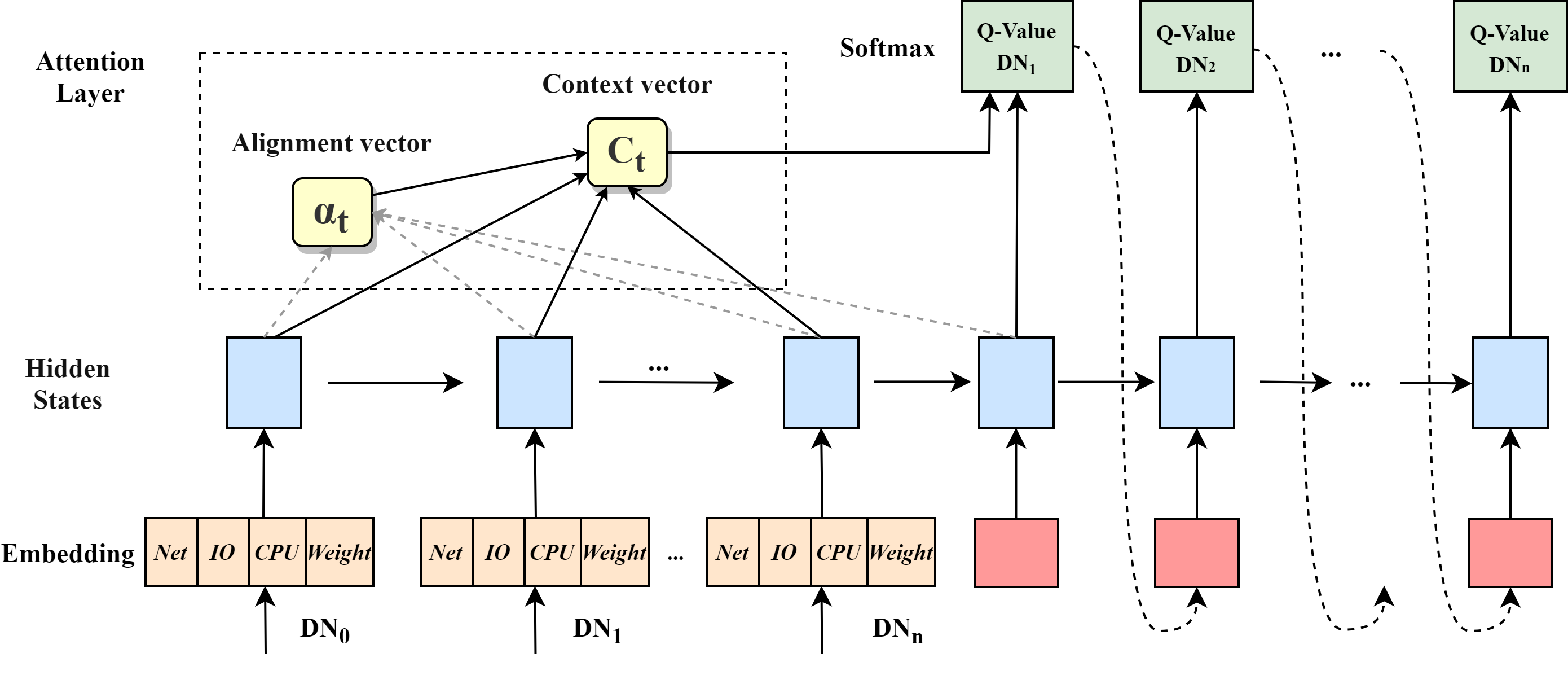
模型的输入是前面定义的State集，被存储为可调的嵌入向量，它可以处理各种数量的数据节点。同时LSTM 在计算的过程中可以得到每个数据节点的隐层状态。该译码器是一个固定时间步长的注意LSTM模型，与输入序列的译码步数相同。

The inputs to this model are the previously defined state set, which are stored as tunable embedding vectors. The sequence model LSTM can handle a variety of data nodes. And LSTM can obtain the hidden layer state of each data node in the process of calculation. The decoder is an attentional LSTM model which has the same number of decoding steps as the input sequence. At each step, the decoder outputs the Q-value with the action (DN), which is the same as the MLP in Placement Agent. Attention mechanism calculates alignment scores between the previous decoder hidden state and each of the encoder’s hidden states and store scores as the alignment vector. And the encoder hidden states and their respective alignment scores are multiplied to form the context vector.

当然在实际应用中，影响系统性能的因素可能更多，对象的访问模式也是有差别的。我们的异构环境较为简单，更详细和复杂的情况在未来的研究中会被考虑。

Of course, in actual applications, there may be more factors affecting system performance, and the object access patterns are also different. Our heterogeneous environment is relatively simple, and more detailed and complex cases will be considered in future work.

Implementation

RLRP是在Park \cite{Park}平台上实现的，这是一个面向学习增强的计算机系统的开放平台。 RLRP的所有代码都是用c++和python编写的，并基于张量流实现了强化学习模型 。此外，RLRP被成功打包到实际的分布式存储系统Ceph (v12.2.13) \cite{Ceph}中。 如图. \ref{Ceph}所示，Mertics收集器和动作控制器通过Ceph Monitor与Ceph交互。 Mertics Collector通过使用Linux SAR (system Activity Report) \cite{SAR}实用程序，每隔30秒从Ceph osd获取系统Mertics。 Action Controller调用Ceph监视器来实现RL Agent所做的放置/迁移操作，并更新Ceph集群的OSDmap。 RLRP以插件的形式实现，并保留了Ceph原有的体系结构和其他流程。

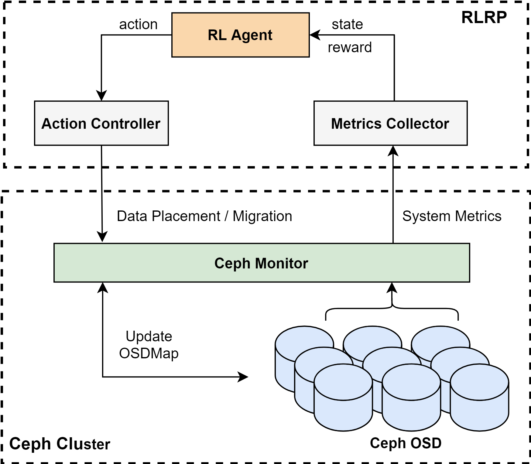
RLRP is implemented on Park \cite{park} platform, which is an open platform for learning-augmented computer systems. All the codes in RLRP are written in C++ and python, and the Reinforcement Learning model is implemented based on the Tensorflow In addition, RLRP is successfully packaged into the actual distributed storage systems, Ceph (v12.2.13) \cite{ceph}. As shown in Fig. \ref{Ceph}, the Mertics Collector and Action Controller interact with Ceph through the Ceph Monitor. Mertics Collector fetches the system mertics from the Ceph OSDs at 30 second intervals by using the Linux SAR (System Activity Report) \cite{sar} utility. The Action Controller invokes the Ceph monitor to implement the placement/migration actions made by the RL Agent and update the OSDmap of Ceph cluster. RLRP is implemented as plug-ins, and retains the original architecture and other processes of Ceph.

Evaluation

1）基于现代分布式存储系统分布算法的标准，RLRP表现如何，和其他算法相比优势是什么？

2）RLRP训练速度如何，训练效果如何？

3）在异构的存储系统中，RLRP优势是什么？

4）在真实的系统和真实负载下，RLRP表现如何？

1) How does RLRP perform based on evaluation criteria of data placement schemes in modern distributed storage systems, and what are its advantages compared with other schemes ?

2) What are the effects of the optimization measures of RLRP on the training with a large number of objects and nodes?

3) What are the advantages of RLRP in heterogeneous storage systems?

4) How does RLRP perform on real-world systems with real workloads?

测试分为仿真系统环境和真实系统环境，前三节的实验在仿真环境中进行，最后一个在真实系统中进行。仿真系统环境基于DaDiSi构建，它是一个用于在(模拟的)存储环境中创建和测试数据分布策略的API 。DaDiSi是一个client-server架构，使用真实负载，通过client端将数据分配到各个server（在DaDiSi种称为disk）中。真实系统环境下的实验是在Ceph中使用rados_bench工作负载来评估RLRP的性能。

另外所有，

环境配置描述如下：

The experiments are carried out in the simulated system environment and the real system environment respectively. The simulation system environment is built on \textbf{DaDiSi} \cite{random,dadisi}, an API for creating and testing data distribution policies in a (simulated) storage environment. DaDiSi is a client-server architecture, and the clinet distributes real-word workload data to each server (Data Node).The experiments in the real system environment is the performance evaluation of RLRP with the rados_bench \cite{rabench} workload in Ceph. In addition, all the experiments are conducted on a local 9-node cluster, one of which is configured as the client node in simulated system environment, and Ceph Admin and Ceph monitor in real system environment. The remaining eight nodes are configured as server nodes (or OSDs in Ceph). Three of them are equipped with an Intel Skylake Xeon Processor (2.40 GHz), 54 GB of memory, and an Intel DC NVMe SSD (P4510, 2 TB); others have Intel Xeon Processor E5-2690 (2.60 GHz) 8-core processors, 16 GB memory and Samsung SATA SSDs (PM883, 3.84 TB) . The operating system running on all nodes is Centos 7 with the kernel of 64-bit Linux 3.10.0.

基于DaDiSi，我们构建了同构和异构两种环境。在仿真同构环境中，所有数据节点在一个服务器上创建，数据节点除了容量上可以设置不同，其他配置完全相同。第一组的性能指标测试在这个环境中进行。仿真异构环境中，每个服务器作为不同的。

Based on DaDiSi, we constructe simulation homogeneous and heterogeneous environments. In the simulation homogeneous environment, all data nodes are created on one server, and the data nodes have the same configuration except for the capacity. In the simulation heterogeneous environment, each server is configured as one data node.

In the simulation homogeneous environment, all data nodes are created on a server, and the configuration of data nodes is the same except for the capacity.

We compare RLRP with other five state-of-the-art schemes. They are 1) Consistent hash.

2) Crush. 3) Random slicing. 4) Kinesis. 5) m

Consistent hash, Crush and Random slicing的实现基于DaDiSI提供的API，Kinesis和m实现基于论文的源码。

In addition, PLRP-pa indicates that RLRP adopts the Placement Agent, PLRP-ma indicates adopting Migration Agent. RLRP-epa and RLRP-ema indicate respectively adopting Placement Agent and Migration Agent , which use the placement model for heterogeneous environment.

DaDiSi为每个数据节点分配不同数量的大小为1Tdisk来模拟容量大小，在初始阶段，有100个节点（每个节点10个disks，10TB），每次增加100个容量不等的节点（每个节点10~15个disks，10~15TB），第三组增加100个10~20TB的节点，以此类推，最后总共500个节点。每个对象大小为1MB，在每一组是进行10^4,10^5,10^610^7,10^8个对象进行分配。 另外副本数默认是3，其他将被设置为1~9。我们使用一个元组（Ndata，Nobj，Nk）表示一组实验中数据节点、对象数和副本数的数量，并用x表示变量。实验结果如下：

In the heterogeneous setting, DaDiSi puts a different number of 1T hard disks to each data node to simulate the capacity. The experiments begin with 100 same data nodes (10 disks per node, 10TB). 100 new data nodes are added in second group, each with capacities varing from 10TB to 15TB. And 100 nodes with 10-20TB capacities are added in the third group, and so on. There are five group experiments, ranging from 100 nodes to 500 nodes. The object size is 1MB, and 10000~10^8 objects are allocated for data nodes in each group. In addition, the default number of replicas is 3 and can be set by different values. We use a tuple (Ndata, Nobj, Nk) to represent the number of data nodes, objects, and copies in a set of experiments, and x to represent variables

The experimental results are as follows:

• 公平性

The distributional fairness is measure with the standard deviation and overprovisioning percentage. For instance, an oversubscription of 10% means that the maximum number of objects is 10% higher than the average.

如图？？和图？？数据是（x，10^6, 3）下的标准差和P。可以看出在RLRP-pa分布效果最佳，数据分布最为公平。标准差比其他算法降低50%以上，且不随数据节点增加而增加。P值略有增加，但也在3%以下。crush，random slicing和kinesis三种基于伪哈希的放置表现也很好，其中kinesis波动较大，主要是因为不同段的哈希函数差别较大。Consistent Hashing表现一般，而DMORP表现最为糟糕，如图右边所示，远远差于其他算法。图？表现了在不同对象数和不同副本数量下的p值变化，可以看到，RLRP-pa非常稳定，P在2%左右，在所有情况表现最佳且波动很小。而crush，random slicing和kinesis，在小数据样本下表现一般，P值为25%~30%，随着数据量或者副本数增加，P值降低到和RLRP-pa接近。而Consistent Hashingp值在5%~20%，在小数据量下表现较好。DMORP依然最差，p值在任何情况下都高于50%。

Figure?? And figure?? show the standard deviation and P under (x, 10^6, 3). It can be seen that RLRP-PA has the most fair data distribution. The standard deviation is more than 50% lower than other schemes and does not increase with the increase of data nodes. The P increase slightly, but it is also below 3%. The pseudo-hash based schemes, Crush, Random Slicing, and Kinesis also perform well and P is 1%~4%. The hash functions of different segments are quite different, which causes the p of Kinesis to fluctuate greatly. Consistent Hashing is mediocre, while DMORP is the worst, as shown on the right, far worse than other schemes . The figure shows the changes of P values under different number of objects and different number of copies. It can be seen that RLRP-PA is very stable with p around 2%, and performs best in all cases with small fluctuation. Crush, random slicing, and kinesis have general performance under small data samples, with a P value of 25% to 30%. As the amount of data or the number of copies increases, the P value decreases to close to RLRP-pa. While Consistent Hashingp value is between 5% and 20%, which performs good under small data volume. DMORP is still the worst, with p-values higher than 50% in any case.

• 时间空间有效性

Time-Space Efficiency} is measure with the memory used in each configuration as well as the performance of each request. Fig. \ref{mtest} shows the average allocated memory over the different tests.

RLRP的内存消耗由agent模型（所有参数）和映射表组成，模型随着节点数（状态空间）增加而增加。但是模型并不是很大，比如100个节点约是2.4M，500节点约是12M。另外由于虚拟节点的设定，映射表比较小，10^6个对象下约为539K。总的来说，和Crush, Random Slicing, and Kinesis 这种去中心化的相比，内存用量会更多，但总体还是很少。 Crush and Kinesis内存消耗非常少，且不受节点数影响，大致为4M左右。Random Slicing当节点增加时需要维护一个表。一致性哈希的内存消耗取决于数据节点的数量，约为40~250M。 DMORP 需要维护额外的信息用于genetic algorithm，内存占用远远大于其他算法且随着数据节点增加而增加，约为1~10G。

The memory consumption of RLRP consists of the agent model (all parameters) and the mapping table. The model increases as the number of nodes (state space) increases. But the model is not very large, for example, the size in 100 nodes is about 2.4m, and about 12M for 500 nodes. In addition, due to the setting of virtual nodes, the mapping table is relatively small, about 539K for 10^6 objects. Decentralized Crush and Kinesis consumes very little memory and is not affected by the number of nodes, which is about 4M. Random Slicing needs keep a small table with information about previous storage system insert and remove operations when the nodes increase, and occupies 4$\thicksim$70M memory. The memory consumption of Consistent Hashing depends on the number of data nodes and is about 40~250M. DMORP needs to maintain additional information for genetic algorithm, which occupies much more memory than other algorithms and increases with the increase of data nodes, about 1-10G.

Consistent Hashing 和 Random Slicing表现最好，只需要5us的时间。RLRP需要大约10us的时间，通过查表。DMORP 和CRUSH都是通过计算的方式，需要20~25us。而Kinesis 需要分段且分段数量随着节点数增加而增加的，每个段的计算方式也不一样，50~160us

• 自适应性

In DaDiSi, a hard disk capacity of 1 TByte and putting 16 hard disks in each shelf means that each data item has a size of 2 MByte. T

In the heterogeneous setting we begin with 100 data nodes, which

• Criteria Evaluation

仿真环境数据节点除了容量上可以不同，其他完全相同

真实系统配置如下，它是一个异构场景，

公平性：标准差，相对权重的标准差来衡量。

Adaptivity

Redundancy: 判断各种算法

High Performance：

查找速度和内存使用率。

1）同构环境中，公平性、适应性、冗余性、内存使用率、查找速率这五个指标来衡量

内存使用率

pool+表

%统计了Stagewise Training和使用大小样本的训练时所用的训练时间和训练效果（R，模型误差），

可以看到，使用小样本训练具有高误差，而大样本训练时间较长。而使用大样本的分段训练既具有较少的误差，训练时间也和小样本训练差不多。

It can be seen that training with small samples has high error, while training with large samples takes longer time. However, the segmented training with large sample has less error and the training time is almost the same as that with small sample.

图？显示了在10~200个数据节点下采用模型方式和普通训练方式下的训练时间，可以明显看到模型的优势所在，比如在20个数据节点下，为了达到很好的训练效果，不优化的训练时间为12247s，而采用模型只需200s，速度提高了98%，且随着数据节点增加提升越明显。

The figure shows the training time under the Model fine-tuning mode and the normal training mode under 10~200 data nodes. You can clearly see the advantages of the model. For example, under 20 data nodes, in order to achieve a good training effect , The unoptimized training time is 12247s, while the model only needs 200s, the speed is increased by 98%, and the improvement is more obvious with the increase of data nodes.

2）异构环境中，会更关注性能

DaDiSi中异构环境只考虑了节点容量的差异，我们对存储的disk，使用真实8个服务器作为存储节点，

• 测试平台：Cloudsim、COSBench、fio/rados benchmark

  https://github.com/intel-cloud/cosbench

• Ceph

• 真实数据

Related Work

传统分布算法

异构环境分布算法优化

RL学习在存储系统中的应用

讨论

• 2021.7.6
• 通用的数据分布的问题基本没什么研究的，问题不够新颖，应该聚焦于具体的未提出未发觉的问题上
• 投稿Transactions on Storage，A类期刊，七月底完成一版

1. 问题不明确：背景中需要增加其他分布方案的问题？

   • 类似于 Random Slicing: Efficient and Scalable Data Placement for Large-scale Storage Systems

   

2. 使用RL的动机不纯？
   • 将分布问题建模，动态分布问题可以看作组合优化问题，RL在解决组合优化问题中发挥出色
3. 迁移方案太过简单，很多因素需要考虑？
4. 方案中增加公式补充？
5. 优化表述不清楚，要结合图详细解释？
6. 测试规模小，osd目前测试到80？至少要扩到100，1000：训练极其慢？
7. 异构考虑较为简单，但是很多动态的不用考虑，应该考虑异构中静态元素。动态元素应当负载均衡考虑？
8. 异构测试效果如何对比说明，需要增加别的方案的测试结果？
9. 测试太少，增加对比测试目标：一致性hash，table-based，crush等等
10. 增加真实系统，真实数据的对比测试
11. 测试补充

• 增加其他分布算法的测试
  • consistent hash：crush：random slicing：table-based：
• 1000 osd的模型训练
  • 放低要求，加速训练
• 封装模型到ceph，真实数据对比测试